BERTopic actor-style matrix

Linking film styles to film makers with BERTopic
This blogpost provides a fully functioning script to: i) open and prepare a dataset; ii) run a model; and iii) retrieve new, useful information from the model’s output.
To work on a project similar to the one discussed in this blogpost, you’ll need a functional Python programming environment. For this I recommend Anaconda, which makes Python programming easier (it comes with many packages pre-installed, helps you to install packages, manage package dependencies, and it includes Jupyter Notebooks, among other useful programs). The remainder of this post assumes that you are working with Anaconda and Jupyter Notebooks. This page will help you to get started with Anaconda, the installation of packages, and Jupyter Notebooks.
Additionally, you’ll need to install the following extra package(s) for the script below to function:
bertopic
The case: Who’s creating which film styles?
Imagine a horror film director who conceives the idea of producing a movie about zombies. The title captures the public’s imagination and becomes a hit, prompting other directors to follow suit. However, over time, audiences may grow weary of the same brain-dead walkers, and interest wanes. The market for this particular style becomes saturated, leading to a decline in production. As audiences seek something fresh, a new stylistic trend has the opportunity to emerge.
In the context of such ‘cultural endogenous’ dynamics (Van Venrooij, 2015; Godart and Galunic, 2019; Sgourev, Aadland, and Formilan, 2023), it is interesting to ask: How do film styles evolve over time? And, how do filmmakers adapt to styles that fall in and out of fashion? Understanding these dynamics could offer valuable insights into how the evolution of styles influences markets for creative works and social life more generally.
To identify distinct styles in films, I use BERTopic (see Grootendorst, 2022, and BERTopic’s homepage) to cluster frequently co-occurring film keywords into topics. The main contribution of this blogpost lies in Sections 3 and 4, where I build on the hierarchical cluster matrix generated by BERT to compute style clusters, generate time series data for these clusters, and link them to the individuals involved in their production. The code can be tested using a small dataset of 3,000 horror films released in the US, which includes both plot-related keywords and information about their creators, as detailed in the next section.
The code
1. Open the dataset
To load a sample dataset on US horror films directly from GitHub, you can use the following Python code. This code utilizes pandas to read the dataset from a GitHub repository URL.
The variables included are: “year,” “title,” and “keywords_list.” Next to this, there is also the “producers_list,” “directors_list,” “writers_list,” “editing_list,” “cinematography_list,” “production_design_list” and “music_departments_list,” who together contitute the “core crew” (see Cattani and Ferriani, 2009).
Please note that some of the code cells’ output has been removed to improve the readability of this blogpost.
import pandas as pd
url = 'https://raw.githubusercontent.com/renswilderom/Various/main/film_keywords.csv'
df = pd.read_csv(url)
print(df.shape)
df.head()
# Merge the people from multiple lists into one "core_crew" column
# These will be the 'actors' in the actor-style matrix


columns_to_process = ['producers_list','directors_list','writers_list','editing_list','cinematography_list','production_design_list', 'music_departments_list']

# Convert string representations of lists to actual lists
import ast
for col in columns_to_process:
    df[col] = df[col].apply(ast.literal_eval)

# Combine lists from all specified columns
df['combined_list'] = df.apply(lambda row: sum([row[col] for col in columns_to_process], []), axis=1)

# Keep rows with 2 or more core crew members (this is relevant for the network analysis, where we are interested in relations between 2 or more people)
import numpy as np
df['len_core_crew'] = df['combined_list'].apply(len)
df = df.loc[df['len_core_crew'] >= 2]
print(df.shape)
df.head()
2. Create a new BERTopic model and visualize it
This section draws on some of illustrative code from BERT’s homepage. The doc_list serving as the model’s input is created from the column with plot-related keywords. Running a BERTopic takes quite a bit longer than, for instance, a conventional LDA topic model. So, it can be smart to save a BERTopic model in order to re-use it at a later point.
# %%time

# Create a new model
# This model uses the default CountVectorizer
# calculate_probabilities=False to speed up the process
# min_topic_size= can be decreased (e.g. to 6) for smaller datasets. By default it is 10.

# Turn the column keywords_list into a list
doc_list = df['keywords_list'].tolist()

from bertopic import BERTopic
from sklearn.feature_extraction.text import CountVectorizer

vectorizer_model = CountVectorizer(stop_words="english")
topic_model = BERTopic(vectorizer_model=vectorizer_model, calculate_probabilities=False, min_topic_size=6)

topics, probs = topic_model.fit_transform(doc_list)
# Get the descriptives as a topic model table
topic_df = topic_model.get_topic_info()
n_topics = topic_df.shape[0]
n_obs = df.shape[0]
topic_df.head()

Now you can visualize the topics with a hierarchical clustering graph that shows the “parent” clusters of each topic. The x-axis in the bottom shows the cosine distance between related topics. For instance, the graph shows that Topic 72 (occult, sorcerer, ritual) is more closely related to Topic 4 (devil, demon, satanic) than to Topic 51 (witchcraft, magic, power) or Topic 66 (Lovecraftian, Paris, sculpture). These four topics are all part of the same parent cluster, with a cosine distance just below 0. This parent cluster can be interpreted as representing a “meta” style within horror films, which is further divided into several substyles (i.e., the individual topics). While some meaningful topics and clusters emerge from these data, it’s important to note that the sample size (n = 3000) is relatively small. A larger dataset or a more fine-tuned BERTopic model could significantly enhance the results.
# Hierarchichal clustering
hierarchical_topics = topic_model.hierarchical_topics(doc_list)
fig = topic_model.visualize_hierarchy()
fig
.png)
3. Unpacking the clusters
This section uses information from the hierarchical cluster matrix generated by BERT. Film titles are linked to specific topics, which are then associated with broader style clusters (i.e., groups of related topics). The data is aggregated yearly to produce time series data for these style clusters.
We begin by using the hierarchical_topics dataframe as input, filtering out all topics/clusters with a cosine distance greater than or equal to 1. Next, we iterate through the remaining clusters, starting with those having the highest distance values. Finally, we remove topics from the list to ensure that each topic is only included in one cluster.
# Compute the hierachical topics
hierarchical_topics = hierarchical_topics[hierarchical_topics['Distance']<1]  # start from distance < 1
hierarchical_topics = hierarchical_topics.reset_index()  # make sure indexes pair with the number of rows
collected=[]
clusters=[]
for index, row in hierarchical_topics.iterrows():
    if (len([i for i in row['Topics'] if i in collected])==0):
        collected.extend(row['Topics'])
        clusters.append([row['Topics'], row['Parent_Name']])
index = 0
for cluster in clusters:
    print(index, cluster)
    index += 1
The code below creates a doc-topic matrix. It shows the probability of each film title being associated with specific topics, indicating the strength of these associations. It is used to determine a cutoff point, identifying whether a film title is “strongly associated” with a particular topic. A “strong” association is defined as a topic probability that exceeds 2 standard deviations (SD) above the mean probability.
# Get the doc-topic matrix
topic_distr, _ = topic_model.approximate_distribution(doc_list)
doctopic=pd.DataFrame(topic_distr)
doctopic
# Calculate the cutoff points
dfm1 = doctopic.describe().loc[['mean','std']]
dfm2 = dfm1.transpose()
dfm2['cutoff_high'] = dfm2['mean'] + dfm2['std'] + dfm2['std']
# dfm2 = dfm2.iloc[:-1]
dfm2.reset_index(level=0, inplace=True)
num_topics=len(dfm2)
dfm2
# Build a dictionary with cutoff points and the column name to make it easier to apply to the dataframe
d = {}
for i, row in dfm2.iterrows():
    d['{}_cutoff_high'.format(i)] = dfm2.at[i,'cutoff_high']

# Use a lambda function to apply the low cutof (the -1 is to exclude the year column)
import warnings
warnings.filterwarnings('ignore')
for column in doctopic.columns:
    doctopic['{}_high'.format(column)]=doctopic[column].apply(lambda x: 1 if x> d['{}_cutoff_high'.format(column)] else 0)
doctopic
# Create a seperate dataframe for the 1/0 doc-topic matrix
doctopic_norm=doctopic.iloc[:, num_topics:]

# Add the clusters
cluster_doctopic_norm = doctopic_norm.copy()

for i in range(len(clusters)):
    cols=[str(x)+"_high" for x in clusters[i][0]]
    cluster_col=cluster_doctopic_norm[cols].sum(axis=1) # sum topics for relevant cluster
    cluster_doctopic_norm['c_{}'.format(i)] = cluster_col

cluster_doctopic_norm = cluster_doctopic_norm.reset_index(drop=False)
cluster_doctopic_norm.head()
# Create a dataframe with clusters only (so omitting the topics)
temp = cluster_doctopic_norm.iloc[:, -len(clusters):]

# Here we turn all the values larger than 1 into 1.
# Hence, a title is either associated with a cluster or not. Titles can can associated with more than 1 cluster.
temp = temp.where(temp == 0, 1)
temp.head()
# Add datetime variable
year = df['year'].values
temp.insert(0, 'year', year)
datetime = pd.to_datetime(temp['year'], errors = 'coerce', format = "%Y")
temp.insert(0, 'datetime', datetime)
temp = temp.drop('year', axis=1)
# Add title
title = df['title'].values
temp.insert(1, 'title', title)
# Add keywords
keywords_list = df['keywords_list'].values
temp.insert(2, 'keywords_list', keywords_list)
temp.head()
# Create time series data
# Group clusters by datetime/year (with the temp dataframe as input)
timeseries={}
for column in temp.columns[1:]:
    timeseries[column]=temp.set_index('datetime').resample('A-DEC')[column].sum()

topic_timeseries_df=pd.DataFrame.from_dict(timeseries)
topic_timeseries_df = topic_timeseries_df.reset_index()
topic_timeseries_df = topic_timeseries_df.drop(topic_timeseries_df.iloc[:, 1:3], axis=1) # drop title and keywords
topic_timeseries_df
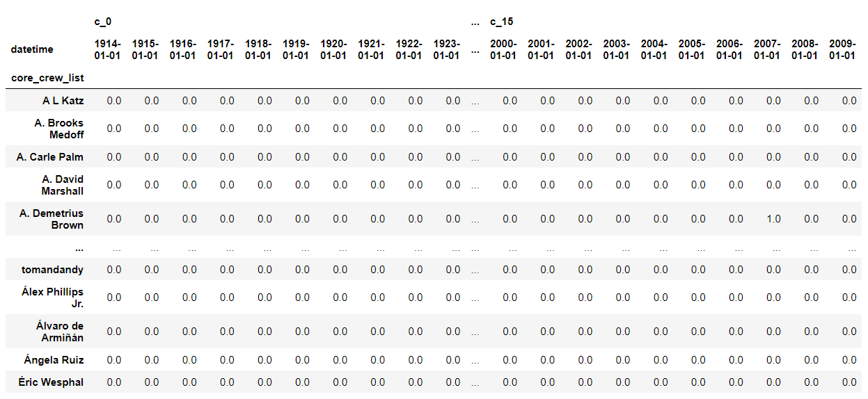
4. The actor-style matrix
With the time series-style data prepared, we can now connect each film’s core crew members to the given styles. The final code cell uses groupby and pivot to generate a dataframe, allowing us to track which filmmakers are linked to particular style clusters in any given year. At this point, it is easy to add more features of the filmmakers (e.g., awards which they received) so that the data can be analyzed using the appropriate methods.
# Add the "core_crew_list" column
actors_matrix=temp.copy()
core_crew_list=df['core_crew']
actors_matrix['core_crew_list'] = core_crew_list.reset_index().drop('index', axis=1)
actors_matrix.head(2)
# Here, the core_crew list is "exploded" meaning that each member and placed on a seperate row
# Duplicates do not have to be removed, since actors are grouped by name and date
exploded_actors_df = actors_matrix.explode('core_crew_list')
exploded_actors_df['core_crew_list'] = exploded_actors_df['core_crew_list'].str.strip() # Strip whitespace to avoid "unique actors" based on a whitespace
print(exploded_actors_df.shape)
exploded_actors_df.head(2)
sum_df = exploded_actors_df.groupby(['core_crew_list', 'datetime']).sum().reset_index()
pivot_df = sum_df.pivot(index='core_crew_list', columns='datetime')
pivot_df = pivot_df.fillna(0)
pivot_df

References
Cattani, G., & Ferianni, S. (2008). A Core/Periphery Perspective on Individual Creative Performance. Organization Science, 19(6), 824—844.
Godart, F.C., & Galunic, C. (2019). Explaining the Popularity of Cultural Elements: Networks, Culture, and the Structural Embeddedness of High Fashion Trends. Organization Science, 30(1), 151-168.
Grootendorst, M. (2022). BERTopic: Neural topic modeling with a class-based TF-IDF procedure. Available at Arxiv.
Sgourev, S., Aadland, E., & Formilan, G. (2023). Relations in Aesthetic Space: How Color Enables Market Positioning. Administrative Science Quarterly, 68(1), 146-185.
Van Venrooij, A.T. (2015). A Community Ecology of Genres. Poetics, 52, 104-123.
Other sources
Photos by Jakob Owens.
